پرونده:Discrete probability distribution illustration.png
پرش به ناوبری
پرش به جستجو
اندازهٔ این پیشنمایش: ۵۳۳ × ۶۰۰ پیکسل. کیفیتهای دیگر: ۲۱۳ × ۲۴۰ پیکسل | ۴۲۶ × ۴۸۰ پیکسل | ۶۸۲ × ۷۶۸ پیکسل | ۹۱۰ × ۱٬۰۲۴ پیکسل | ۱٬۸۰۶ × ۲٬۰۳۳ پیکسل.
پروندهٔ اصلی (۱٬۸۰۶ × ۲٬۰۳۳ پیکسل، اندازهٔ پرونده: ۴۴ کیلوبایت، نوع MIME پرونده: image/png)
| There are SVG versions: | 
|

| |

|
خلاصه
| توضیح |
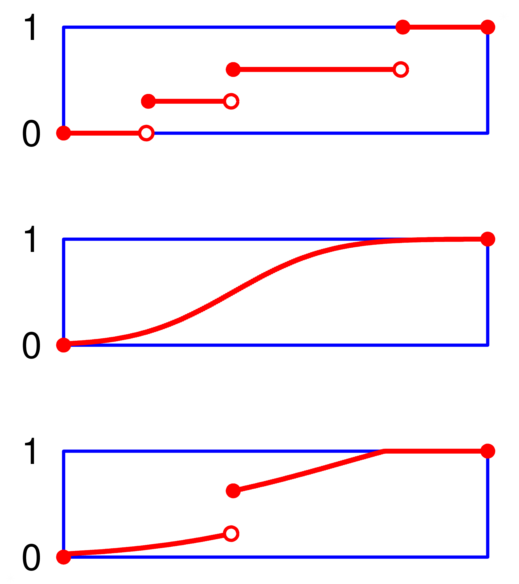
English: From top to bottom, the cumulative distribution function of a discrete probability distribution, continuous probability distribution, and a distribution which has both a continuous part and a discrete part. Cumulative distribution functions are examples of càdlàg functions.
Français : Fonctions de répartition d'une variable discrète, d'une variable diffuse et d'une variable avec atome, mais non discrète.
עברית: בשרטוט העליון מוצגת פונקציית ההצטברות של ההתפלגות הבדידה שלה שלושה ערכים אפשריים: {1}, {3} ו-{7} בהסתברות 0.2, 0.5 ו-0.3 בהתאמה. השרטוט האמצעי מציג את פונקציית ההצטברות של התפלגות רציפה, עובדה שניתן להסיק בשל רציפות הפונקציה על כל הטווח [0,1]. השרטוט התחתון מציג פונקציית הצטברות של התפלגות שהינה רציפה בחלקה ובדידה בחלקה.
Magyar: Az eloszlásfüggvények például càdlàg függvények.
Italiano: Le funzioni di ripartizione sono un esempio di funzioni càdlàg.
日本語: 上から順に、離散確率分布、連続確率分布、連続部分と離散部分がある確率分布の累積分布関数.
한국어: 이산 확률 분포, 연속 확률 분포, 이산적인 부분과 연속적인 부분이 모두 존재하는 분포에 대한 각각의 누적 분포 함수.
Polski: Od góry: dystrybuanta pewnego dyskretnego rozkładu, rozkładu ciagłego, oraz rozkładu mającego zarówno ciągłą, jak i dyskretną część.
Српски / srpski: Одозго на доле, функција расподеле дискретне случајне променљиве, непрекидне случајне променљиве, и случајне променљиве која има и непрекидне и дискретне делове.
Sunda: From top to bottom, the cumulative distribution function of a discrete probability distribution, continuous probability distribution, and a distribution which has both a continuous part and a discrete part.
Türkçe: Yukarıdan aşağıya doğru: bir ayrık olasılık dağılımı için, bir sürekli olasılık dağılımı için ve hem sürekli hem de ayrık kısımları bulunan bir olasılık dağılımı için yığmalı olasılık fonksiyonu. Üsten alta doğru. Bir aralıklı dağılım için, bir sürekli dağılım için ve hem sürekli bir kısmı hem de aralıklı bir kısmı bulunan bir dağılım için yığmalı dağılım fonksiyonları.
Українська: Зверху вниз: функція розподілу для дискретного розподілу ймовірностей, для неперервного розподілу та для розподілу що містить дискретну та неперервну частини.
Tiếng Việt: Từ trên xuống dưới, hàm phân phối tích tũy của một phân phối xác suất rời rạc, phân phối xác suất liên tục, và một phân phối có cả một phần liên tục và một phần rời rạc. Hàm phân bố tích lũy là một ví dụ của hàm số càdlàg. |
| منبع | اثر شخصی |
| پدیدآور | Oleg Alexandrov |
| دیگر نسخهها | see above and below |

|
File:Discrete probability distribution illustration.svg یک نسخهٔ برداری از این پرونده است.
آن پرونده را هنگامی که بهتر بود میبایست به جای این نسخهٔ تصویر استفاده کرد. File:Discrete probability distribution illustration.png → File:Discrete probability distribution illustration.svg
برای کسب اطلاعات بیشتر در ارتباط با تصاویر برداری لطفاً اینجا را مطالعهکنید. همچنین اطلاعات بیشتری در ارتباط با حمایت مدیاویکی از تصاویر اسویجی وجود دارد. |
 |
اجازهنامه
| من، دارنده حق تکثیر این اثر، این اثر را به مالکیت عمومی منتشر میکنم. این قابل اجرا در تمام نقاط جهان است. در برخی از کشورها ممکن است به صورت قانونی این امکانپذیر نباشد؛ اگر چنین است: من اجازهٔ استفاده از این اثر را برای هر مقصودی، بدون هیچگونه شرایطی میدهم، تا وقتی که این شرایط توسط قانون مستلزم نشده باشد. |
Source code (MATLAB)
% plot a the cummulative distribution function for a
% (a) discrete distribution
% (b) continuous distribution
% (c) a distribution which has both a discrete and a continuous part

function main()

   clf; hold on; axis equal; axis off;
   L=4; h = 0.02;
   X=0:h:L;
   shift = 2;

   Y = [0*find(X < 0.2*L), 0.3+0*find( X >= 0.2*L & X < 0.4*L) 0.6+0*find(X >= 0.4*L & X < 0.8*L), 1+0*find(X>= 0.8*L)];
   plot_graph(X, Y, L, 0*shift)

   Y = 0.5*erf((4/L)*(X-L/2.5))+0.5;
   plot_graph(X, Y, L, shift);

   ds = 0.4;
   Y = 0.5*erf((2/L)*(X-L/1.5))+0.5;
   Y = Y + [0*find(X < ds*L) 0.4+0*find(X >= ds*L)]; Y = min(Y, 1);
   plot_graph(X, Y, L, 2*shift);

   % plot two dummy points to make matlab expand a bit the window before saving
   plot(L+0.15, 1.1, '*', 'color', 0.99*[1, 1, 1]);
   plot(-0.5, -2.1*shift, '*', 'color', 0.99*[1, 1, 1]);

   % save as eps
   saveas(gcf, 'Discrete_probability_distribution_illustration.eps', 'psc2')

function plot_graph(X, Y, L, shift)

   % settings
   N = length (X);
   tol = 0.1;
   thick_line = 3;
   thin_line = 2;
   small_rad = 0.07;
   red= [1, 0, 0];
   blue = [0, 0, 1];
   fs = 23;
   epsilon = 0.01;

% plot a blue box
   plot([0, L, L, 0, 0], [0, 0, 1, 1, 0]-shift, 'linewidth', thin_line, 'color', blue)

   % everything will be shifted down
   Y  = Y - shift;

   % if the given funtion has a jump, plot some balls. Otherwise plot a continous segment
   for i=1:(N-1)
      if abs(Y(i)-Y(i+1)) > tol

	 ball       (X(i+1), Y(i+1), small_rad,                red);
	 empty_ball (X(i),   Y(i),   thin_line, 0.9*small_rad, red);

      else
	 plot([X(i)-epsilon, X(i+1)+epsilon], [Y(i), Y(i+1)], 'color', red, 'linewidth', thick_line);
      end
   end

   ball       (0, -shift, small_rad,             red);
   ball       (L, 1-shift, small_rad,             red);

%plot text
   small= 0.4;
   text(-small, 0-shift, '0', 'fontsize', fs)
   text(-small, 1-shift, '1', 'fontsize', fs)


function ball(x, y, r, color)
   Theta=0:0.1:2*pi;
   X=r*cos(Theta)+x;
   Y=r*sin(Theta)+y;
   H=fill(X, Y, color);
   set(H, 'EdgeColor', 'none');


function empty_ball(x, y, thick_line, r, color)
   Theta=0:0.1:2*pi;
   X=r*cos(Theta)+x;
   Y=r*sin(Theta)+y;
   H=fill(X, Y, [1 1 1]);
   plot(X, Y, 'color', color, 'linewidth', thick_line);
تاریخچهٔ پرونده
روی تاریخ/زمانها کلیک کنید تا نسخهٔ مربوط به آن هنگام را ببینید.
| تاریخ/زمان | بندانگشتی | ابعاد | کاربر | توضیح | |
|---|---|---|---|---|---|
| کنونی | ۱۲ مهٔ ۲۰۰۷، ساعت ۱۶:۵۱ | | ۱٬۸۰۶ در ۲٬۰۳۳ (۴۴ کیلوبایت) | wikimediacommons>Oleg Alexandrov | {{Information |Description= |Source=self-made |Date= |Author= User:Oleg Alexandrov }} Made with matlab. {{PD-self}} |
کاربرد پرونده
صفحهٔ زیر از این تصویر استفاده میکند: